42 conditional formatting data labels excel

How to Create Excel Charts (Column or Bar) with Conditional Formatting Conditional formatting is the practice of assigning custom formatting to Excel cells—color, font, etc.—based on the specified criteria (conditions). The feature helps in analyzing data, finding statistically significant values, and identifying patterns within a given dataset. Excel Data Analysis - Conditional Formatting - Tutorials Point Follow the steps to conditionally format cells − Select the range to be conditionally formatted. Click Conditional Formatting in the Styles group under Home tab. Click Highlight Cells Rules from the drop-down menu. Click Greater Than and specify >750. Choose green color. Click Less Than and specify < 500. Choose red color.

Excel tutorial: How to add a conditional formatting key That way, we can adjust the conditions for the rules using the key itself. The first step is to create the basic layout for the key. For this, we'll set up a small table with three rows - one for each conditional format. We can then add labels for each conditional format rule. These could be anything, but let's use Excellent, Concern, and ...

Conditional formatting data labels excel

Conditional Formatting of Excel Charts - Peltier Tech Feb 13, 2012 · It’s relatively easy to apply conditional formatting in an Excel worksheet. It’s a built-in feature on the Home tab of the Excel ribbon, and there many resources on the web to get help (see for example what Debra Dalgleish and Chip Pearson have to say). Conditional formatting of charts is a different story. Conditional Formatting - Tableau Different than excel, conditional formatting in Tableau cannot be applied across a column but rather across a mark. Marks are generated when measures are added to the rows/columns shelf. Adding these additional marks allows a user to achieve a similar result to excel-like conditionally formatted crosstabs. See below for the steps required to ... How to create a chart with conditional formatting in Excel? Add three columns right to the source data as below screenshot shown: (1) Name the first column as >90, type the formula =IF (B2>90,B2,0) in the first blank cell of this column, and then drag the AutoFill Handle to the whole column;

Conditional formatting data labels excel. Excel Conditional Formatting Data Bars Select the cells that contain the data bars. On the Ribbon, click the Home tab. In the Styles group, click Conditional Formating, and then click Manage Rules. In the list of rules, click your Data Bar rule, then click the Edit Rule button. In the "Edit the Rule Description" section, the default settings are shown for Minimum and Maximum. Conditional Formatting - Tableau Different than excel, conditional formatting in Tableau cannot be applied across a column but rather across a mark. Marks are generated when measures are added to the rows/columns shelf. Adding these additional marks allows a user to achieve a similar result to excel-like conditionally formatted crosstabs. See below for the steps required to ... Change the format of data labels in a chart To get there, after adding your data labels, select the data label to format, and then click Chart Elements > Data Labels > More Options. To go to the appropriate area, click one of the four icons ( Fill & Line, Effects, Size & Properties ( Layout & Properties in Outlook or Word), or Label Options) shown here. Conditional Formatting in Excel (In Easy Steps) 1. Select the range A1:A10. 2. On the Home tab, in the Styles group, click Conditional Formatting. 3. Click Highlight Cells Rules, Greater Than. 4. Enter the value 80 and select a formatting style. 5. Click OK. Result. Excel highlights the cells that are greater than 80. 6. Change the value of cell A1 to 81. Result.

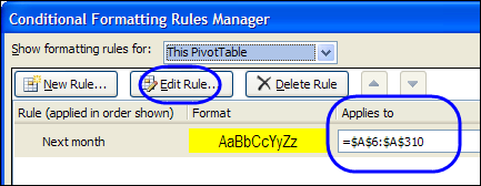
How to Apply Conditional Formatting to Pivot Tables - Excel … 13.12.2018 · Conditional Formatting can change the font, fill, and border colors of cells. It can also add icons and data bars to the cells. The formatting will also be applied when the values of cells change. This is great for interactive pivot tables where the values might change based on a filter or slicer. How to Setup Conditional Formatting for Pivot ... Conditional Formatting For Blank Cells | (Examples and Excel Always use limited data to deal with and apply bigger conditional formatting to avoid excel getting freeze. Recommended Articles. This has been a guide to Conditional Formatting for Blank Cells. Here we discuss how to apply Conditional formatting for blank cells along with practical examples and a downloadable excel template. You can also go ... Excel bar chart with conditional formatting based on MoM change Click on the Select Data button on the Chart Design ribbon to open the Select Data Source dialog box. In the list of Series, select the Label spacer series and use the arrows to move it to the top of the list (this places it behind all other series on the chart). Click on the Label spacer bar and on the Chart Format ribbon set the Shape Fill to ... How to do conditional formatting of a label in Excel VBA I need to format a label value conditionally in "$K" and "$M" when the data is in thousands and millions. I've been using the following format which works absolutely fine in Excel cells ($#,##0.0,"K") and ($#,##0.00,,"M") respectively, this doesnt work when I use it to format a label caption using VBA with the following code :

Excel Conditional Formatting not functioning correctly after … 10.01.2018 · Everything works fine, formatting changes according to changes in the data! Now I copy a range of sheet A to sheet B using VBA, that works OK. However: in sheet B the conditional formatting of these cells is not working correctly anymore: > cells using 'format only cells that contain' work correct! formatting changes correctly when data changes Conditional Formatting to Distinguish Between Labels and Numbers I want to conditionally format each cell, so that the text is yellow, the numbers are blue, and the blank cells are green. I tried by setting up a new rule under conditional formatting, then selecting "use a formula to determine which cells to format", then using some combinations of the if, istext, isnumber, etc. combinations. Please advise. Creating Conditional Data Labels in Excel Charts - YouTube We can make labels appear on our charts that don't have to do with the raw numbers that built the chart - and we can make them show up or not based on whatever conditions we want. In this tutorial,... Conditional formatting of chart axes - Microsoft Excel 2016 To change the format of the label on the Excel 2016 chart axis, do the following: 1. Right-click in the axis and choose Format Axis... in the popup menu: 2. On the Format Axis task pane, in the Number group, select Custom category and then change the field Format Code and click the Add button: If you need a unique representation for positive ...

Format Cells using Conditional Formatting in Excel

Changing the Color of a Data Label using IF Statement 1) Click on the data labels to highlight all the data labels, 2) Right-Click and select Format Data Labels, 3) Click on Number, 4) Go to the Format Code field *adapt the following to your needs* 5) [green] [>29]#.00; [<30] [Color 53]#.00 Click to expand... Hi Jawnne, I hope you're still lurking about on here.

conditional formatting - Getting Excel to Conditionally Copy Data to Another Sheet - Super User

Progress Doughnut Chart with Conditional Formatting in Excel 24.03.2017 · Great question! The Excel Web App does not support those text box shapes yet. We can use the built-in data labels for the chart instead. The label for the Remainder bar can be deleted by left clicking on the label twice, then pressing the delete key. That just leaves the data label for the actual progress amount. Here is a screenshot.

[SOLVED] Conditional copying data into another sheet

How to change chart axis labels' font color and size in Excel? Sometimes, you may want to change labels' font color by positive/negative/ in an axis in chart. You can get it done with conditional formatting easily as follows: 1. Right click the axis you will change labels by positive/negative/0, and select the Format Axis from right-clicking menu. 2.

Format Pivot Table Labels Based on Date Range – Excel Pivot Tables

Conditional formatting for Data label colors at li ... - Power BI When using conditional formatting for data labels, as introduced in July 2021, the overall number is used for the calculation, instead of the line number average.. Using "data colors > default color > fx" gives the expected behavior.Bars with an average value above 50 are green, others red: However, when choosing "data labels > color > fx", the same setup results in all data labels shown in a ...

How to Create Multi-Category Chart in Excel - Excel Board

VBA Conditional Formatting of Charts by Value and Label To run the procedure, select the chart, then press Alt+F8, select FormatPointByCategoryAndValue, and click Run. VBA Conditional Formatting of Charts by Series Name. VBA Conditional Formatting of Charts by Value. VBA Conditional Formatting of Charts by Category Label. Conditional Formatting of Lines in an Excel Line Chart Using VBA.

SQL Workbench/J User's Manual SQLWorkbench

New Conditional Formatting experience in Excel for the web 20.01.2022 · Formula – you can now specify the formatting criteria using a logical formula in Excel for the web. This rule type gives you the added flexibility of formatting a range based on the result of a function or evaluate data in cells outside the selected range. Formula rule type . More coming soon to Conditional Formatting in Excel for the web:

Stacked Bar Chart Data Labels Outside - Free Table Bar Chart

How to Apply Conditional Formatting to Rows Based on ... - Excel Campus On the Home tab of the Ribbon, select the Conditional Formatting drop-down and click on Manage Rules…. That will bring up the Conditional Formatting Rules Manager window. Click on New Rule. This will open the New Formatting Rule window. Under Select a Rule Type, choose Use a formula to determine which cells to format.

Conditional Formatting in Excel

Conditional Formatting in Excel - a Beginner's Guide Click Conditional Formatting, then select Icon Set to choose from various shapes to help label your data. For this example, let's use the arrow icon set to show whether our highlighted data, the Variance column, has increased or decreased. Now, you'll see that the data has arrow icons accompanying their values in the cells.

Conditional Copy Data from One sheet to another workbook - Excel VBA / Macros - OzGrid Free ...

Progress Doughnut Chart with Conditional Formatting in Excel Mar 24, 2017 · Great question! The Excel Web App does not support those text box shapes yet. We can use the built-in data labels for the chart instead. The label for the Remainder bar can be deleted by left clicking on the label twice, then pressing the delete key. That just leaves the data label for the actual progress amount. Here is a screenshot.

Basic Conditional Formatting in Excel and Access | ExcelDemy

How to Apply Conditional Formatting to Pivot Tables - Excel ... Dec 13, 2018 · Conditional Formatting can change the font, fill, and border colors of cells. It can also add icons and data bars to the cells. The formatting will also be applied when the values of cells change. This is great for interactive pivot tables where the values might change based on a filter or slicer. How to Setup Conditional Formatting for Pivot ...

Excel Conditional Formatting Help - www.hardwarezone.com.sg

Conditional formatting chart data labels? - Excel Help Forum The easy way to conditionally format these labels is use two series. Use something like =IF ($E2=1,0,NA ()) for the series that has red labels and =IF (#E2=1,NA (),0) for the series that has unformatted labels. Jon Peltier Register To Reply Bookmarks Digg del.icio.us StumbleUpon Google Posting Permissions

Excel Course: Inserting Graphs

How To Use Conditional Formatting in Excel in 5 Steps Excel separates each group with a vertical line and labels at the bottom of the group. Finally, click on the "Conditional Formatting" button. 4. Select an option from the drop-down menu Once you select the "Conditional Formatting" button, Excel displays several options, starting with "Highlight Cells Rules" and ending with "Manage Rules."

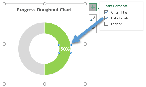
Progress Doughnut Chart with Conditional Formatting in Excel - Excel Campus

Excel Conditional Formatting not functioning correctly after ... Jan 10, 2018 · Everything works fine, formatting changes according to changes in the data! Now I copy a range of sheet A to sheet B using VBA, that works OK. However: in sheet B the conditional formatting of these cells is not working correctly anymore: > cells using 'format only cells that contain' work correct! formatting changes correctly when data changes

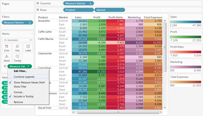
Tableau Legends Per Measure and Conditional Formatting Like Excel

Custom Chart Data Labels In Excel With Formulas Follow the steps below to create the custom data labels. Select the chart label you want to change. In the formula-bar hit = (equals), select the cell reference containing your chart label's data. In this case, the first label is in cell E2. Finally, repeat for all your chart laebls.

How to Create a MS Excel Pivot Table – An Introduction | SIMPLE TAX INDIA

Tom’s Tutorials For Excel: Conditionally Formatting Locked … In the Conditional Formatting dialog box, click OK, and you are done. IF YOU ARE USING EXCEL VERSION 2007 OR AFTER: Step 5 (version 2007 or after) — Press Alt+O+D to show the Conditional Formatting Rules Manager dialog box: • In the “Show Formatting Rules for” field, select Current Selection. • Click on the item labeled “New Rule”.

How to Copy Conditional Formatting in Excel

Excel Conditional Formatting in Pivot Table - EDUCBA But there is a loophole with the condition formatting here. Whenever we make any changes in the Excel Pivot data, then conditional formatting will not be applied to the correct cells, and it might not include the whole new data. The reason being is when we select a particular cell range for applying conditional formatting in excel. Here we have ...

Share :